Pandemic Flu Spread Using “Green” Simulation Method for Small Sample of Elementary Students
Authors: Carlos Ordonez and Juan Carlos Pineda
Abstract: This paper studies a pandemic flu spread case applying a “green” simulation method, using pseudo-random numbers as presented in the paper by Wilson S., Alabdulkarim A. and Goldsman D. W, “Green Simulation of Pandemic Disease Propagation” (Wilson S., 2019) in a simulation environment built in Python. The scenario is an elementary school with twenty-one kids and the impact of infection when one infected kid enters the system. The findings and answers to the questions are presented in this paper.
- Background and Description of the Problem
The novel Coronavirus pandemic has affected how the world operates, limiting our ability to mobilize and interact within each other. Throughout the history of humankind there have been several endemic and pandemic viruses that have attacked our society (Morens DM, 2009;200(7)), and researchers have study and implemented models to understand how the viruses spread among the population. For this paper the susceptible-infected-removed (SIR) model is used. The SIR model states that an individual at time t could change between three different states, susceptible (S), infected (I), and removed (R) (Morens DM, 2009;200(7)) (Munkhbat, 2019).
This paper analyzes the case of an elementary school with twenty-one students having one infected child on the first day. The infection rate β = 3 as the infected kid can infect on three consecutive days. The probability of infecting any other kid is p=0.02 and it is modeled using Bernoulli independent, identically distributed p trials. As a new kid becomes infected, he or she will have the same 3-day infection rate and the same p probability to infect other children.
For this simulation we will be using a simplified approached not considering any mitigation effect through social distance, or more complex models. The simplified approach is based on the “green” method presented in the paper by Wilson (Wilson S., 2019) that reuses many Bernoulli p trials between runs of susceptible individuals. The first section describes the setup of the environment. The second section describes the result with different iterations and answers to the questions such as the distribution of infection of Day1 , the expected number of kids infected on Day 1, the expected number of kids infected by Day 2 and a histogram detailing the length of the pandemic.
-
Main Findings
- Modeling
The SIR model is a mechanistic description of the spread of infectious disease. Each parameter is a state defined by differential equations that model the observed data at any given time t. The state susceptible refer to the individual that could be exposed to an infected person. Infected is the person that acquired the disease. Removal are individuals that either recovered or dead.
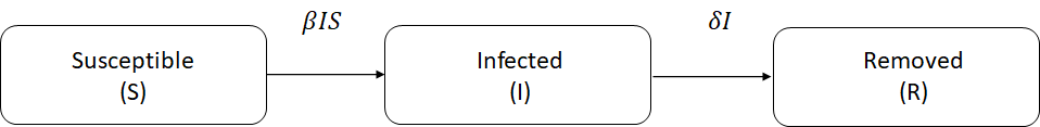
Figure 1. SIR Model block diagram
The differential equations 1a,1b, 1c describes each of the models from the Figure 1.

Susceptible individuals will transition to the infected state at a rate of β and then will continue transition to the removed at a rate δ. This model is widely used in large populations. As presented by Wilson (Wilson S., 2019), the use of differential equation model tends to perform poorly in a setting with a small population. Also, he points out that additional short comings of this model do not take randomness into account and individual level behavior.
A better approach as Wilson et al. (Wilson S., 2019), proposed, is the use of discrete-event simulation, using a “green” simulation technique, where individuals enter in contact with each other and with the infected individual, and the outputs from the results of the previous days are being reused. This technique was introduced by Staum et. al (Feng & Staum, 2015), and fits the model of the 21 elementary students in the project. Using a simplified version of the SIR model, we are simulating susceptible random individuals that may be infected by “Tommy”, the infected individual, at most once per day. Having a probability of infection p, each encounter being independent, therefore meeting the requirement of having encounters as Bernoulli trials. The simulation will end when no more susceptible individuals will get infected or no more susceptible individual will remain. The simulation runs for different sets of independent replications to calculate the expected number of kids infected, and to answer the questions presented in the project.
- Setup of the Simulation Environment
The simulation starts by generating uniform - Unif (0,1) - pseudo-random numbers (PRN) U for each susceptible individual for each day per each replication. Twenty (20) PRNs are created for each susceptible kid on Day 1 and compared to the probability of infection p = 0.02. There is one super-infective kid, “Tommy”, which is represented as I(0)=1 arriving to the school on the first day. The number of susceptible at the beginning of Day 1 is represented by S(0)=20 and the number of removals R(0)=0. Tsai, et al. (Tsai, et al., 2010) proposed a way that all the k infectives entering the room, interacts with all n susceptible, by means of Bern(p) trials. Then, the probability of a susceptible becoming infected is equal to 1 - qk with q = 1 – p. Therefore, performing n Bern(1 - qk). For example, on Day 1 the probability of p*(t=1) = 1-(1 - 0.02)1 = 0.02. It is important here to highlight, that as each day passes the probability changes depending on the number of k infected kids. The simulation will have a Bern(p*(t)) trials and will end when no more kids are infected. The number of k infected kids per day is calculated by comparing p*(t) < U and updating the value of p* every day. On Day 2 PRNs are calculated for the remaining susceptible children and so on until no additional kid gets infected. To give another example, in order to calculate Day 2, assuming that result of the PRN for the end of the Day 1 is 2 infected, p = 0.02, the Day 2 will start with S(2) = 19, I(2)=2 including “Tommy”, p*(2)= 1 - ( 1 - 0.02)2 = 0.0396, R(0)= 0 and so on. The problem establishes that infected individuals will remain infected for a δ of three days, therefore “Tommy” will change from “infected” to “removed” on Day 4, for our example R(4)=2.
- Modeling and Results
Table 1 shows how the states from the SIR model changes, the probability and the number of cumulative PRNs generated from Day 1 until no additional children gets infected for the first replication. On Day 1 there is 1 infected, “Tommy” = I(1), with S(1) = 20 susceptibles, R(1) = 0 recovered, a probability p*(1)=0.02, with total number of PRNs generated, and a total number of PRNs= 20 (Cumulative PRNs) . Day 2 shows s one additional infected for a total of I(2) =2, S(2)= 19, R(2) = 0, the new p*(2)=0.0396, total cumulative PRNs= 40. On Day 4 we see the first removed, “Tommy”. As the days progress, we stop seeing new infections Day 6 and the last infected person gets removed on Day
- Therefore the spread of infection ends on Day 10 with a total infected of I(10)=9 kids and S(10)=12 susceptible that did not get infected.
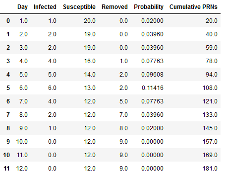
Figure 2 shows the first replication using a stack plot where can be seen how the infection susceptible and removed individuals change status over time for the 21 kids with a 3 day infection rate, and a probability of infection of p=0.02.
The peak of the of the number of infected individuals happened on Day 5. On Day 6 started to die down until the spread stopped on Day 9 where the last kid was removed or recovered. The total of susceptible/not-infected individuals were 12, and the total of infected individuals were 9.
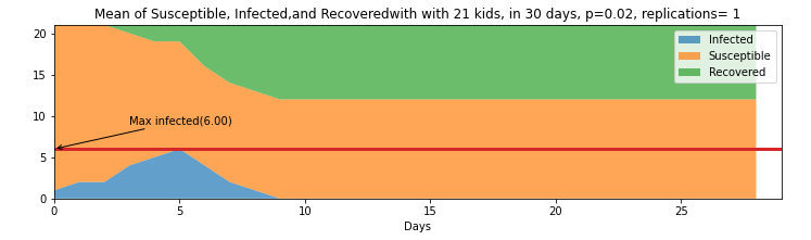
Figure 2. Stack plot of 21 kids with 30 days for the first replication
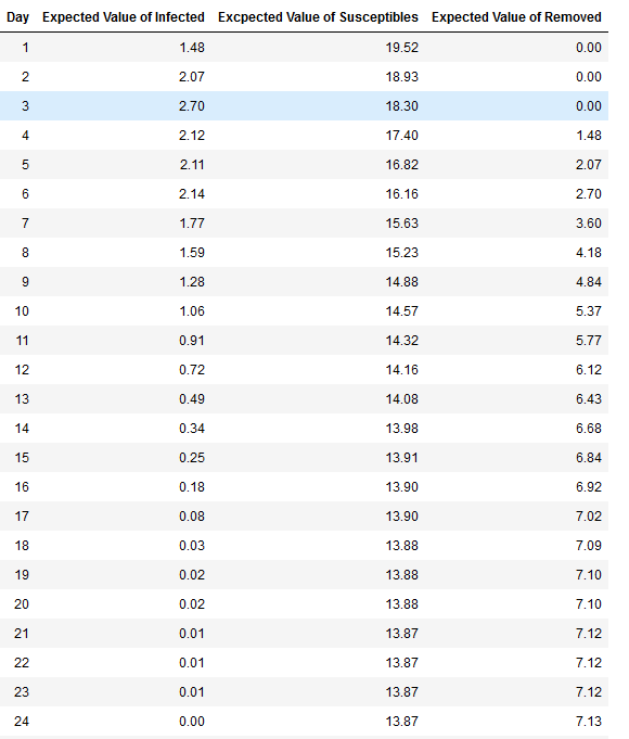
Figure 3, shows the next step, running 100 replications of this same scenario and finding the expected value of the status per day to understand how the model behaves using the same base parameters. The top part shows the stacked plot of the expected value of each day for the different status. On the bottom part of the same figure is an expanded view of the rate of infections and the variance. The figure shows that on average the day with most infections is Day 3. Additionally, it shows that on average the infections end on Day 24. Table 4 on the Appendix section shows the value of each day for the different status (infected, susceptible, and removed)
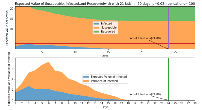
Figure 3. Top: Expected value of status per day with 21 kids in 30 days p=0.02 and 100 replications. Bottom : Expected value and variance of infected per day with 21 kids in 30 days p=0.02 and 100 replications
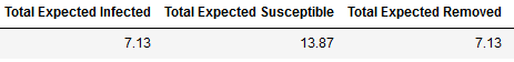
Taking the expected value for each of the three status after 100 replications, in average 7.13% of students get infected, 13.87% of students remain susceptible, and 7.13% gets removed. Table 2 presents the restuls. We can imply that about 7 kids get infected and 14 kids do not. The variance as seen in orange on the bottom graph of Figure 3, has it highest pick on Day 6 with a pick of 5.15 and expected value of 1.77 , implying that number of kids infected for that Day 6 could change between 2 to 5. This could be the result of having a three (3) day infection rate.
The following histograms on Figure 4 shows where most of values fall after the 100 replications. It can be seen that at least one person gets infected most of the time, which is obvious since the system is initialize with Tommy, the infected kid. After that, it varies between two to six following what looks like a geometric distribution considering that we are doing the number of Bernoulli trials until the first success. The recovered distribution seems to follow also a geometric distribution and the susceptible values complement recovered ones.
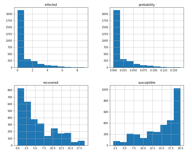
Figure 4. Histograms of infected, recovered/removed, susceptible and the probability after 100 replications
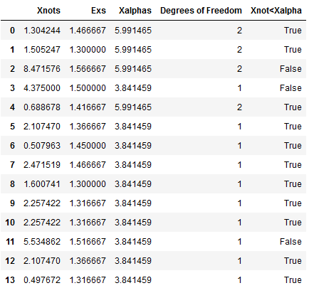
To validate that the values for Day 1 corresponded to a geometrically distribution, we performed a goodness of fit with a group of smaller values of n=60 for replications 1 to 990 in batches, with a total number of batches equals to 14 batches. We encountered that 11 times out of 14 our χo was smaller than the χα at 0.95. Resulting that it is very likely that the distribution for the first day fits the geometric. Results of the 14th batch is shown below. Table 5 in the Appendix shows the total results per batch.
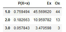
Figure 5. 14th Batch results for Goodness of fit.
-
Answer to the questions presented in the Project
- What is the distribution of the number of kids that Tommy infects on Day 1?
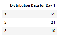
After taking the values of m=100 replications and plotting the results, we realized there are at least one kit kid gets infected 69% of the time. Similarly, at least 2 kids get infected 21% of the time and at least 3 kids get infected 10% of the time for the 100 replications reflected on Table 2.

Therefore, the distribution for Day 1 as presented in the histogram of Figure 3 shows a geometric distribution.
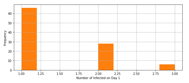
Figure 6. Distribution for Day 1
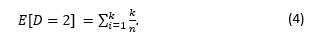
- What is the expected number of kids that Tommy infects on Day 1?
The expected number of kids that Tommy infects on Day 1 can be defined:
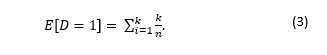
The result is equal to 1.48.
- What is the expected number of kids that are infected by Day 2 (you can count Tommy if you want)?
Similarly, the expected number of kids that are infected on Day 2 is equal to 2.07
- Simulate the number of kids that are infected on Days 1,2,. . . . Do this many times. What are the (estimated) expected numbers of kids that are infected by Day i, i = 1, 2, . . .? Produce a histogram detailing how long the “epidemic” will last.
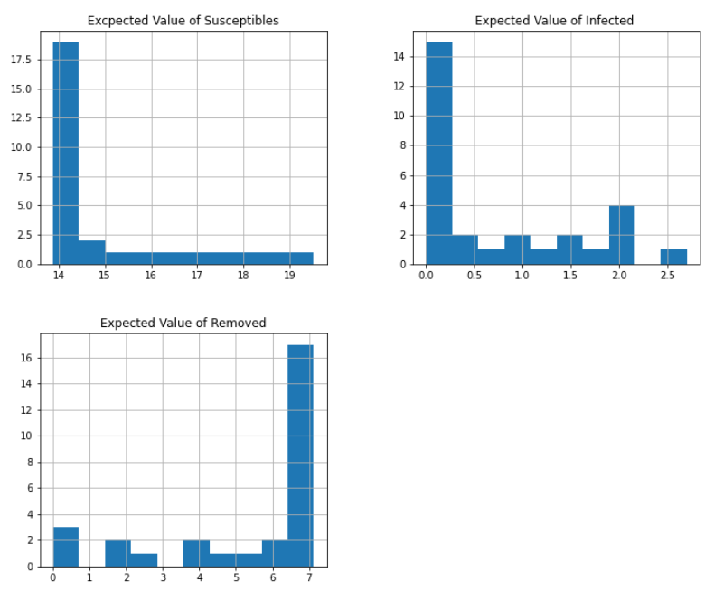
Figure 7. Histogram of expected value per status
After running the simulation for 100 times (m=100) and taking the expected value for each status per day, we see that the infected values approximate to a geometric distribution. As can be seen in the histograms below on Figure 6. The Expected Value of Susceptible and Expected Value of Infected kids are likely to follow a geometric distribution. The Expected value of the removed roughly fits a skewed normal distribution, which is an encouraging result as is similar to the one presented by Disworh (Disworth, 2019).
The values of the Expected Value of removed kids and the Expected value of the infected can be seen as a “mirror” because as the days progress, the kids that get infected become removed.
- Conclusions
After reading all the material on Pandemic and/or Disease transmission we learned the way how these problems are modeled. SEIR and SIR models are used to capture the process of the infection. The SEIR model is more general, however for our solution we picked the SIR model as described by Wilson et al (Wilson S., 2019) due to its simplicity way of modeling by means of Bernoulli process.
One key takeaway of the simulation is that even though the model is simple, implementing it has to be done carefully since generating PRN’s in a large number of replications can be costly from the computing stand point. This Is very important and we noticed it after growing our replication number from 10, to 100 to 1,000 and then further from that.
Once we determined the right length of the spread of the virus, the “green” simulation technique used for this project becomes computationally efficient. The “green” simulation technique considers a probability that reuses many Bernoulli p trials between runs of susceptible individuals, updating the rate of infected induvial between consecutive days. The results showed that in average the pandemic lasted k= 24 days after m= 100 replications, with n= 20 susceptible kids exposed to 1 infected on Day 1. It also resulted that the total number of expected kids I(t) = 7 infected a including Tommy; and the total S(t) =14 susceptible kids, after some rounding. The distribution of the infected individuals after the m=100 replication for Day 1 is likely to be geometric. The same is the case for the distribution of the expected values of infected kids. The variance peaked on Day 6, which could be due to the three days that infected kids continue spreading the virus.
Finally, this simulation shows a simplified way to get acquainted with using PRNs to estimate the rate of infections. Further work could include factoring the use of social distance or other means that could help mitigate the infection rate. Portions of the code can be found here.
References
Disworth, M. (2019, January 2). Infecting Modeling - Part 1. (Towards Data Science) Retrieved from https://towardsdatascience.com/infection-modeling-part-1-87e74645568a
Feng, M., & Staum, J. (2015). Green simulation designs for repeated experiments. In Proceedings of the 2015 Winter.
Morens DM, F. G. ( 2009;200(7)). What is a pandemic? . J Infect Dis., 1018-1021.
Munkhbat, B. (2019). A Computational Simulation Model for Predicting Infectious Disease Spread using the Evolving Contact Network Algorithm. Master Thesis.
Tsai, M., Chern, T., Chuang, J., Hsueh, C., Kuo, H., Liau, C., . . . Shen, C. (2010). Efficient simulation of the spatial transmission dynamics of influenza. PLoS ONE, 5, e13292.
Wilson S., A. A. ( 2019). Simulation of Pandemic Disease Propagation . Symmetry, 11(4), 580.
Appendix