Data Analysis and Prediction of Waterpoint Functionality Using Spatial and Non-spatial Machine Learning Models
Data Analysis and Prediction of Waterpoint Functionality Using Spatial and Non-spatial Machine Learning Models
Georgia Tech OMSA Practicum with ESRI
Carlos Ordonez, Rozsa Zaruba
December 1st, 2021
Abstract
The main purpose of this project is to apply the knowledge obtained during the Master’s in Analytics by way of using ESRI’s ArcGIS Pro spatial software and their Python API, ArcPy. The learning process was through a project that analyses water point data in Uganda. With ESRI’s team guidance, we were set on a learning adventure. We learned how to manipulate our data in ArcGIS, how to transfer the code into Jupiter notebooks, how to think spatially, and use layers to better extract information. We were able to see the differences (both advantages and disadvantages) between traditional Python programming and ArcPy. At the end, we used our knowledge to build classification models to be able to tell if a water point is functional or not. Finally, we used ESRI’s story map to create a presentation of our findings.
The interactive map can be found here: Uganda Water Point Analysis - Storymaps
Introduction
Having clean and safe water, is a basic necessity that we take for granted. Unfortunately, many rural areas in the World have no easy access to water. Most of Uganda’s population live in rural areas and two third of them lack easy access to safe water. Women and children spend most of their day walking back and forth between water source and home.
People in many developing worlds walk an average of 3.7 miles a day for water. Some parts in Uganda if people want to access clean water, the only reliable borehole is about this distance one way. It can take between 90 minutes to two hours to walk that distance. Boreholes sometime serve more than 850 people, which makes them incredibly crowded. You could wait two to three hours because of long lines . This has an impact on everybody’s life: women cannot get jobs, children cannot go to school, etc. Having water access does not guarantee that is safe to consume, creating a health impact to society. The lack of infrastructure and access to clean potable water in Uganda is one of the factors slows their progress1
Problem Statement
This project analyses the water point data set for Uganda from the Water Point Data Exchange (WPDx) using ESRI’s ArcGIS Pro and their Python API. The project aims to find relationships in the dataset that might explain why certain places do not have access to water, with the final goal of finding a model that can predict the functionality of a water points.
Data
-
Water Point Data Exchange (WPDx)2 where waterpoint data are a set of records that uniquely identify water points and provide additional attributes such as the type and condition of the infrastructure, functionality, service levels, etc.
-
ESRI provided additional data sets:
-
World Population Estimate for 2016
-
Africapolis urban area dataset
-
Enrichment data for Uganda from arcgis.geoenrichment3
-
Data Cleaning
Our original dataset had 121,472 observations on 52 features. The provided dataset for Uganda contained points outside the country’s boundaries. After removing the points outside, the total observation remaining were 118,110. The dataset also contained many redundant columns: e.g. “management_clean”, “management_original” and “management”, containing the same data. We kept the ones we thought would be most informative for our study.
Examining the data further, we noticed that more than 80% of the data in the “water_tech_clean” was labeled as “NaN”. It was decided not to impute data for this attribute in our study, because most of the variables are categorical, and all of them have multiple levels (management has 137 levels) and it would muddy our results. Our solution was to remove the missing values. For “water_tech”, that would mean reducing our data drastically. Reading up on the variables, we realized that “NaN” is the base line for this variable, and it means that there is no technology in place. E.g., there is a river and people would just use their jugs to fill it up with water. Our solution was to change the variables to “Notech” value and use it as one of the levels in the variable.
Taking advantage of ArcGIS Pro, we were able to add a new categorical variables to our dataset such as “Type_of_Region” describing if the point observation is considered to be in an urban or rural area.
##
Data Exploration:
For the data exploration portion, we are going to answer questions as provided in the scope of the project to try to understand more about the data.
- Which district has the most non-functional water points?
For the project, it was determined that ”F_status_id” provides information about the functionality of the water point. For this question, the approach is to work with non-functional data and obtain the districts in percentage with the largest number of non-functional water points.
Figure 1. Heatmap of non-functional water points per district as percentage of the total non-functional waterpoints, being the district of Wakiso the largest with a total of 930 or 4.36% of the total non-functional.
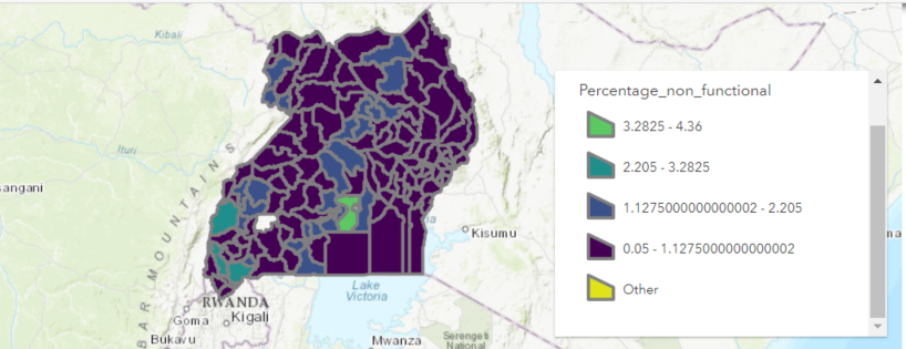
Figure . Heatmap of non-functional water points per district as percentage of the total non-functional waterpoints
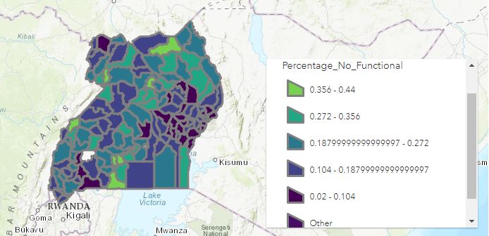
Figure . Heatmap of non-functional water points as percentage of total waterpoints per district
Figure 2 shows the percentage of non-functional waterpoints as a portion of the total functional and non-functional waterpoints per districts having the district of Pakwach the largest with 44.08% being non-functional as per Figure 3.
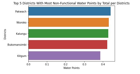
Figure . Top 5 Districts with most non-functional waterpoints per district totals
- What are the top causes of non-functional water points?
Analyzing the causes of non-functional water points the initial approach was to understand what type of labeling the attribute “F_status” had on each point. Table 1 shows that 90.76% has “Non-functional” label.
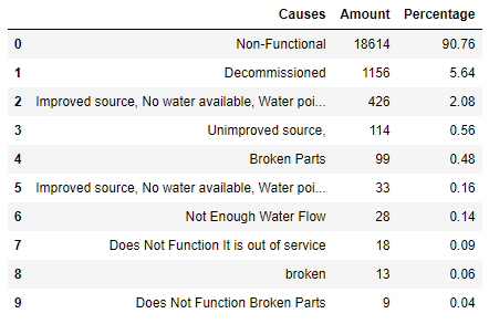
Exploring further, it was found that out of the 18,614 non-functional water points, there are 14,914 “Community Management” equivalents to 80.12% of total non-functionals. Furthermore 3,973 of those non-functional charged a fee. It is possible to assume that the community managing the water points does not have the means to be able to support the infrastructure necessary to treat them, and the Government cannot reach those communities in order to provide a service in which they could charge. Also, it is possible that the poverty level of those communities does not allow them to pay for water service.
- Which year saw the most water point installations?
Doing a bar plot analysis as per Figure 4 it was found that 2007 was the year with the highest water point installations. There is a clear increase after 1986, which makes sense if we consider the country’s history. Uganda had a Civil War between 1980 till 1986. People started going back to their homes, there was need for more water, and the country tried to recover from the war.
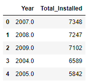
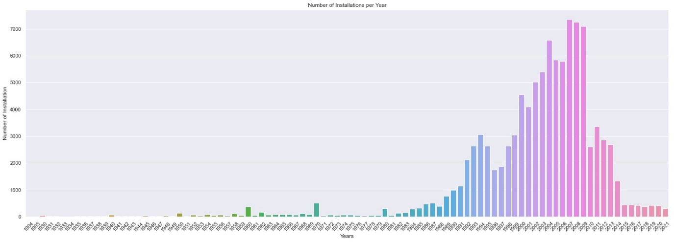
Figure Number of installations per year
- Which water points serve the largest rural population? Repeat the analysis for urban population. Do these water points have anything in common?
Using spatial filtering techniques with “Uganda_UrbanAreas_Africopolis” as the filter, a new attribute was created to determine rural and urban water points. Then with the layer “Uganda_Pop2016_points_clipped” a boundary of 1km was established outside the urban areas. We established a large population by finding the mean of the population, that was established at 436 per population point as shown on Figure 5. Figure 17 in the Appendix shows the distribution of the population and the mean.
Figure . Waterpoints serving the largest urban and rural populations
- Is there a relation between age of water point and the water point being Non-functional?
When we are looking at the summary of the data for functional and non-functional water points based on the installation year, we get a false sense that in recent installation years we have more broken points. In reality, there are more water points installed recently than in the past. We divided up the data into two intervals: water points installed before 1985 we consider old, everything after is new. Based on the histogram 1985 looked like a natural break, new point installations picking up after. As we mentioned above, this aligns with the country’s history too.
We calculated the percentage of non-functional water points for the old and new installations. We found that 27.6% of the old water points were non-functional, while “only” 18.5% of the new wells were broken. To answer the question, yes the older the water point it is more likely that it may be broken.
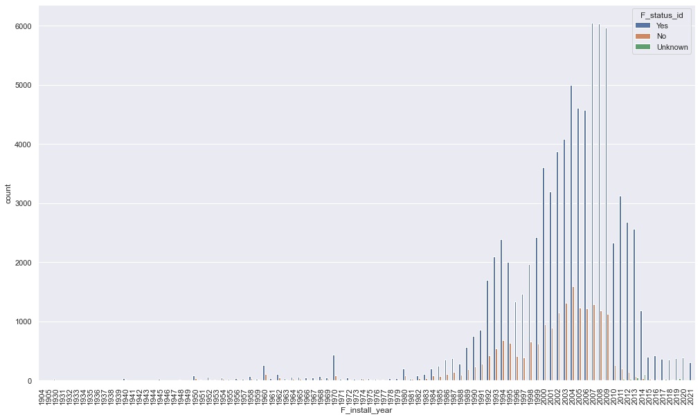
Figure Installation per year with functionality
- Which district has the largest number of old water points serving the highest rural population?
After aggregating the points by districts for the largest water points of the rural areas, the district of Ntungamo shows the largest number of points. The graph shows the values in percentages. Ntungamo is the green district in the south of the country in Figure 7.
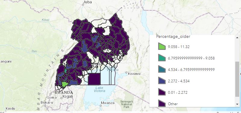
Figure Heatmap of districts with largest old waterpoints serving highest rural populations
The top five districts with largest old waterpoints serving the highest rural populations are shown on Figure 8
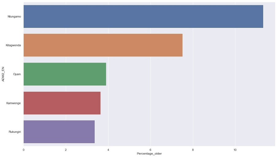
Figure Heatmap of top 5 districts with largest old water points serving highest rural populations
- Is there an association between water source, water tech, facility type or management for Non-Functional water points?
Using aggregate numbers for each of these variables can be misleading. For example, boreholes have the greatest number of non-functioning water points. But most of the water points are boreholes. We decided to use percentages again to see the relationships better. Our Findings:
-
As a result, 20.85 % of the “undefined shallow wells are broken. The number of “protected shallow wells” and “piped water” are much smaller to fairly compare to the boreholes, but it is still alarming that 23% of them is broken
-
23% of the hand pumps are broken
-
Only 17% of the water points is broken if the facility type is improved. It jumps up to 29% for unknown or 24% if there is no facility.
-
Private operators have only 7% of broken water points. Community management and Other Institutional Management are doing fairly with 19% and 25% broken points. All the other managements do poorly maintaining the water points, school management being the worst with 81% of broken water points.
Another way to look at association between variables is to look at the correlation matrix as per Figure 9. The correlation matrix does not show high correlations. To see how significant the relationships are we did a chi-square analysis with the following null and alternative hypothesis:
H_0: There is no association between pairwise variable.
H_Alt: There is significant association.
Our p-values are very large, which tells us that we cannot reject the null hypothesis, there is no significant association between variables.
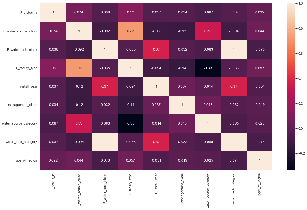
Figure Correlation matrix of selected attributes
We have to note that the correlation matrix and chi-square analysis both assume linear relationship. Our conclusion thus is that there is no linear association between variables, we need to find models that handle non-linear relationships (like Random Forest) and avoid the ones that assume linear relationships (like Logistic Regression).
- What percent of the population does not have easy access to working water points?
This question was answered entirely using ArcPy and ArcGIS Pro. We created 1 km buffers and counted all the points that fall outside of it as shown in Figure 10. The total number of population outside of a 1km radius of functional water points is 7,010,728. This is equivalent to almost 20% of Uganda’s population (for the year of 2016).
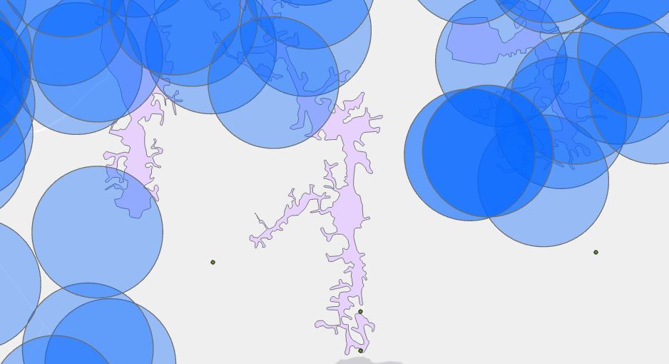
Figure 1Km buffer in blue to aggregate counts of waterpoints outside the border
GeoEnrichment and Imputation
Our results in the previous sections did not show a clear relationship between variables. To improve our dataset, we decided to enrich the data. We connected with the online ArcGIS tool to enrich the data for every district. One of the challenges that we encountered is that the enriched data had fewer districts than the one in our dataset. This created a series of null values in several districts. To overcome this, we impute information based on the location of the district. This was accomplished by finding the districts in the vicinity of the missing district and taking the average of the enriched parameters. Figure 11 shows in darker colors the districts that had no enrichment information and the districts that were used for imputation around them in a lighter color.
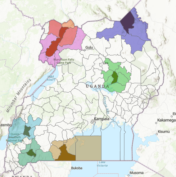
Figure Districts in dark have requires impute with neighbor districts in lighter color
The KeyFacts in the GeoEnrichment library contained potentially valuable information for the country and the districts. Some of the available variables were unemployment, population density, number of males, number of females, etc.
The enriched data showed promising attributes, but many of them were correlated with each other. By removing the highly correlated attributes and leaving the ones that explain the data better, a new dataset was created with the following variables:
| F_lat_deg | Latitude information (used in spatial analysis) |
|---|---|
| F_lon_deg | Longitude information (used in spatial analysis) |
| F_status_id | Yes/No Working and non-working water points |
| F_water_source_clean | Categorical: 13 unique values |
| F_facility_type | Categorical: improved/unimproved |
| F_install_year | Installation year |
| management_clean | Categorical: reduced to 9 unique values |
| water_source_category | Categorical: reduced to 7 unique values |
| water_tech_category | Categorical: 4 unique values |
| Type_of_region | 0/1: Rural/Urban |
| Age | old/new |
| ADM1_EN | Eastern/ Northern/ Central/ Western |
| UNEMP_CY | Unemployment from key facts |
| POPPRM_CY | Population per million |
| AVGHHSZ_CY | Average household size |
Table Causes of non-functionality
Feature Extraction
As we saw above, it is hard to find a meaningful explanation between variables. It does not mean that there is none, it only means that there is no linear association. Clustering would find points that are similar to each other, so it is a good method for feature extraction. We explore a couple of techniques and save results as features for our classification analysis.
Our non-spatial clustering method is KModes clustering. It is one of the unsupervised Machine Learning algorithms that is used to cluster categorical variables (with categorical variables we cannot calculate the distance as we would do with Kmeans algorithm). This method uses the dissimilarities (total mismatches) between the data points. The lesser the dissimilarities the more similar our data points are. It uses modes instead of means.
The KModes images show points with similarities. To the naked eye it is difficult to assess what similarities they have. Our intent with this clustering technique is to use it for modeling as features (variable in the dataset is Cluster_KModes).
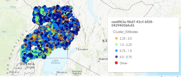
Figure KModes spatial representation
We explored three different spatial clustering techniques such as: Hierarchical Density-Based Spatial Clustering of Applications with Noise (HDBSCAN), Ordering Points To Identify Cluster Structure (OPTICS), and Spatial Constrained Multivariate Clustering.
HDBSCAN is a powerful algorithm that uses Density-Based Spatial Clustering of Applications with Noise (DBSCAN), converting it into a hierarchical clustering algorithm, and then using a technique to extract a flat clustering-base in the stability of clusters. Densities are estimated based on core distances and form the density landscape. Using a global threshold to set the sea level at, DBSCAN identifies the “islands“ (DBSCAN). Then HDBSCAN helps decide: are these several “islands” or one “island” with multiple peaks? Figure 13 shows a representation of HDBSCAN clusters and the output was saved as a feature for modeling. The gray color represent noise. Figure 19 shows cluster allocation.
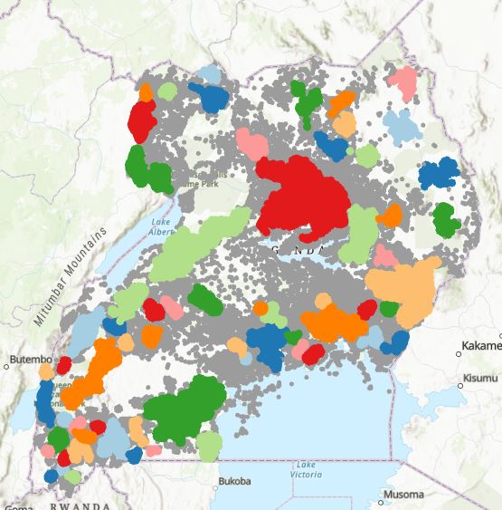
Figure Clustering using HDBSCAN
OPTICS is a technique that has two principles: Core Distance and Reachability Distance. Core Distance is defined as the minimum value of radius required to classify a given point as a core point. If the given point is not a Core point, then its Core Distance is undefined. The Reachability Distance: is defined with respect to another data point. This clustering technique is different from other clustering techniques as it does not explicitly segment the data into clusters. Instead, it produces a visualization of Reachability distances and uses this visualization to cluster the data. The resulting clusters are visualized in Figure 14. The blue cluster represents the large allocation of a cluster. Figure 20 shows the cluster allocation. Figure 21 shows the reachability plot. After further examination we noticed that HDBSCAN and OPTICS have a 99.5% correlation. For our future analysis we decided not to use the OPTICS results as it would not add extra information to our models.
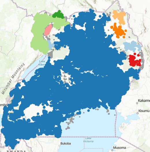
Figure Clustering using OPTICS
Spatial Constrained Multivariate Clustering: This is an unsupervised machine learning method that finds spatially contiguous clusters of features based on a set of attribute values and optional cluster size limits. Figure 15 shows the result. Our interpretation is that points are being cluster by latitude and longitude and installed year. The goal of using this method is to help our algorithm determine which algorithm help improve our modeling.
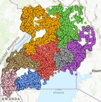
Figure Spatially Constrained Multivariate Clustering
Dimensionality Reduction
Dimensionality reduction helps compress the data with less noise. We can use the reduced data for our modeling. Two methods were explored: Multiple Correspondence Analysis and Autoencoder Neural Network.
Correspondence Analysis (CA) is a Dimensionality Reduction technique that is traditionally applied to contingency tables. It transforms data in a comparable manner as Principal Component Analysis (PCA), where the central result is a Singular Value Decomposition (SVD). CA needs the data to be in contingency tables which means it is more appropriate to apply it to categorical features. Multiple Correspondence Analysis (MCA) is an extension of the CA for more than two categorical features (three or more). We have more than two categorical features, hence the use of MCA. We ran MCA on our data reducing the features to the first 2 components.
Autoencoder is an unsupervised artificial neural network that compresses the data to lower dimensions and then reconstructs the input back. Autoencoder finds the representation of the data in a lower dimension (middle layer) by focusing more on the important features getting rid of noise and redundancy. We are going to use this middle, compressed layer as features in our modeling.
Data used for modeling:
For most of our analysis, we used the reduced enriched dataset with clustering information. We also explored a dataset with only the MCA components and clustering information, another with only autoencoder features and clustering information. For more details see Appendix.
Proposed Methodology for Analysis
The main question that we would like to answer is: Can we predict the status of a water point (working or non-working)? This is a classification problem. Classification usually refers to any kind of problem where a specific type of class label is the result to be predicted from the given input field of data.
We approached the problem in two ways: Through spatial analysis and non-spatial analysis. For non-spatial analysis, KNN, Naïve Bayes (NB), SVM, Random Forest are used from Python’s scikit-learn library. For spatial analysis, we use Random Forest Classifier from ArcPy package.
To have a base reference we are running a dummy classifier (only identifies majority class labels), but we are also using Naive Bayes as a baseline. It does not make sense to do a logistic regression as the data exploration did not suggest a linear relationship. Our main focus is going to be on K-Nearest Neighbor (KNN), Support Vector Machines (SVM) and Random Forest models.
*Naïve Bayes* (NB) classifier is a probabilistic classifier based on Bayes’ theorem, which assumes that each feature makes an independent and equal contribution to the target class. NB classifier assumes that each feature is independent and does not interact with each other, such that each feature independently and equally contributes to the probability of a sample belonging to a specific class.
K-Nearest Neighbor (KNN) is a supervised and pattern classification learning algorithm that helps find which class the new input belongs to when k nearest neighbors are chosen and distance is calculated between them. It attempts to estimate the conditional distribution of Y given X, and classify a given observation to the class with the highest estimated probability. We found the optimal number of neighbors using the elbow method. Each model for each dataset was tuned individually and the number of k that minimized error rate was chosen for each model as shown in Figure 18.
Support vector machine (SVM) is a linear model for classification and regression problems. It can solve linear and non-linear problems and work well for many practical problems. The idea of SVM is simple: the algorithm creates a line or a hyperplane which separates the data into classes. For our data this may not be the best solution as this method cannot create nonlinear separations.
Random Forest is a classification algorithm consisting of many decisions trees. It uses bagging and feature randomness when building each individual tree to try to create an uncorrelated forest of trees whose prediction by committee is more accurate than that of any individual tree. We are using grid search to find the optimal setup for each dataset. The decision metric for the grid search is ‘ROC-AUC’.
Metrics Used for Evaluation
Confusion Matrix is a performance measurement of the classification.
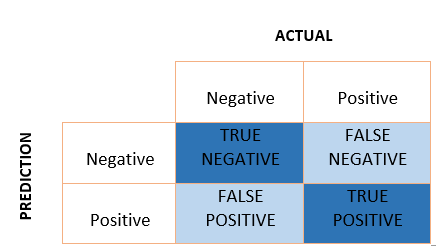
Figure Confusion Matrix Illustration
The Kappa Coefficient: Cohen’s Kappa is defined as (Observed Accuracy - Expected Accuracy) / (1 - Expected Accuracy). It evaluates how well the classification performs compared to chance, in which all values are just randomly assigned. The coefficient ranges from -1 to 1 and a value greater than 0 indicates that the classification is significantly better than random. This metric was used between non-spatial models.
Precision — Measures what percent of your predictions were correct. Precision can be defined as the ability of a classifier not to label an instance positive that is actually negative. For each class, it is defined as the ratio of true positives to the sum of a true positive and false positive.
Recall — Measures what percent of the positive cases did you catch. Recall is the ability of a classifier to find all positive instances. For each class it is defined as the ratio of true positives to the sum of true positives and false negatives.
F1 score — Measures what percent of positive predictions were correct. The F1 score is a weighted harmonic mean of Precision and Recall such that the best score is 1.0 and the worst is 0.0. F1 scores are lower than accuracy measures as they embed Precision and Recall into their computation. As a rule of thumb, the weighted average of F1 should be used to compare classifier models, not global accuracy.
AUC (Area Under the ROC curve) — Represents the degree or measure of separability. It tells how much the model can distinguish between classes. The higher the AUC, the better the model is at predicting classes correctly. AUC is scale-invariant: it measures how well predictions are ranked, rather than their absolute values. Also, AUC is classification-threshold-invariant: It measures the quality of the model’s predictions irrespective of what classification threshold is chosen.
Dealing With Unbalanced Data
Before starting the modeling, we examined the data for class distribution, and we noticed that the two classes are heavily unbalanced: only 19% of the data belongs to the minority class (non-functional water points). The challenge of working with imbalanced datasets is that most machine learning techniques will ignore, and in turn have poor performance on, the minority class, although typically it is performance on the minority class that is most important. Some of the classical solutions would be to use methods that train on the majority class and identify minority classes as an anomaly. Two methods were tried in our study:
-
One-Class SVM: When modeling one class, the algorithm captures the density of the majority class and classifies examples on the extremes of the density function as outliers.
-
Isolation Forest is a tree-based anomaly detection algorithm. It is based on modeling the normal data in such a way to isolate anomalies that are both few in number and different in the feature space. Tree structures are created to isolate anomalies: isolated examples have a relatively short depth in the trees, whereas normal data is less isolated and has a greater depth in the trees.
Having unbalanced data made us consider different over and under-sampling techniques too. We are creating data sets with over-sampling, under-sampling and over-and-under sampling at the same time. We kept a separate testing set and only over/under-sample the training data. We train the models on this data and use the separate testing data for testing.
Oversampling Techniques
One approach to addressing imbalanced datasets is to oversample the minority class. The simplest approach involves duplicating examples in the minority class, although these examples do not add any new information to the model. We call this traditional oversampling.
Synthetic Minority Oversampling Technique (SMOTE) synthesizes new examples from the existing examples. There are variations of this approach:
-
SMOTE works by selecting examples that are close in the feature space, drawing a line between the examples in the feature space, and drawing a new sample at a point along that line. Specifically, a random example from the minority class is first chosen. Then k of the nearest neighbors for that example is found (typically k=5). A randomly selected neighbor is chosen, and a synthetic example is created at a randomly selected point between the two examples in feature space.
-
Borderline-SMOTE is an extension to SMOTE, it involves selecting those instances of the minority class that are misclassified, such as with a k-nearest neighbor classification model. We can then oversample just those difficult instances, providing more resolution only where it may be required.
-
Borderline-SMOTE SVM: Instead of k-nearest neighbor, it uses an SVM. Also, the technique attempts to select regions where there are fewer examples of the minority class and tries to extrapolate towards the class boundary.
Under-sampling Methods
Under-sampling is a technique to balance uneven datasets by keeping all of the data in the minority class and decreasing the size of the majority class. We tried the following variations:
-
NearMiss-1: Selects only those majority class examples that have a minimum distance to three minority class instances, defined by the n_neighbors argument.
-
Tomek Links: If the examples in the minority class are held constant, the procedure can be used to find all of those examples in the majority class that are closest to the minority class, then removed.
-
Edited Nearest Neighbors Rule for Undersampling: This rule involves using k=3 nearest neighbors to locate those examples in a dataset that are misclassified and that are then removed before a k=1 classification rule is applied.
-
One-Sided Selection for Undersampling: It is an undersampling technique that combines Tomek Links and the Condensed Nearest Neighbor (CNN) Rule.
-
Neighborhood Cleaning Rule for Undersampling: It combines both the Condensed Nearest Neighbor (CNN) Rule to remove redundant examples and the Edited Nearest Neighbors (ENN) Rule to remove noisy or ambiguous examples. It focuses less on improving the balance of the class distribution and more on the quality (unambiguity) of the examples that are retained in the majority class.
Random Over-and-under Sampling
These techniques use both over and undersampling together to create the training dataset. First, they are oversampled and undersampled right after. Variations that we used:
-
Random over than undersampling
-
SMOTE-TOMEK
-
SMOTE and Edited Nearest Neighbors
Analysis and Results
Summary of Non-Spatial Results
We ran many models with different data sets and are comparing the best of them. More detailed outputs can be found in the Appendix.
Our dummy classifier (a classifier that only finds the majority label) has an average accuracy of 81%. This is already a sign why not trust this metric since we already know that it does not capture any of the minority cases. The AUC curve is 0.5, the Cohen Kappa is 0, telling us that this is not a useful model.
Our other base model is the Naïve Bayes: the best model we found was for the sample that was SMOTE oversampled and Nearest Neighbor undersampled at the same time. AUC curve improved to 0.58, Cohen Kappa 0.103 which suggests that the model is somewhat useful. We also look at the precision and Recall numbers, especially we are interested in the minority class. With a higher Recall but low Precision, our classifier considers that more points are non-functional than they are.
Support Vector Machine: We were getting some promising Precision results (see Table 4), but the Recalls were very much close to 0. If we did not care about false negatives, and we only focused on true positives and false positives this high Precision result may even be good. But this is another question because we do not have a cost analysis to associate to the model. Which one costs more? Going out to repair a wrongly classified working well, or not going out to a non-working well? Models need high Recall when we need output-sensitive predictions and we need to cover false negatives as well. If it is okay to flag working wells as not working but a non-working wells should not be flagged as working then we would need a high Recall. The F-1, Cohen Kappa and AUC on the other hand suggested that this model is not good.
**Sample Autoencoder and clusters** precision recall f1-score support 0 0.80 0.00 0.01 4941 1 0.81 1.00 0.89 20486 accuracy 0.81 2542 macro avg 0.80 0.50 0.45 25427 weighted avg 0.80 0.81 0.72 25427 Cohen Kappa: 0.005 AUC: 0.502 |
|---|
Table 5 largest waterpoints installation per year
Adding the cluster information to our base enriched data did not improve significantly our models. Same for using MCA and Autoencoder Neural Network reduced datasets. One-class classification methods did not seem to work better either. We started seeing some changes with over/under sampling techniques. We used the enriched dataset with cluster information to create new samples on the training data. We ran most of the models (except for the one-class models) and saw that the AUC moved above 0.60, the precision and Recalls are closer to each other. We chose the traditional oversample results (Table 5) to be able to compare it with the spatial analysis and because it got slightly better results. The rest of the sampling methods created synthetic data and we cannot create coordinate data with them to be able to use it in spatial analysis.
Model Sample traditional oversample |
Precision | Recall | F-1 | Cohen Kappa | AUC | Accuracy | |||
|---|---|---|---|---|---|---|---|---|---|
| Status_id | 0 | 1 | 0 | 1 | 0 | 1 | |||
| KNN k=3 | 0.56 | 0.79 | 0.55 | 0.8 | 0.55 | 0.79 | 0.347 | 0.672 | 0.72 |
| Naïve Bayes | 0.3 | 0.81 | 0.05 | 0.97 | 0.08 | 0.88 | 0.029 | 0.51 | 0.79 |
| Support Vector Machine | 0.65 | 0.74 | 0.28 | 0.93 | 0.39 | 0.82 | 0.249 | 0.606 | 0.72 |
| Random Forest | 0.66 | 0.79 | 0.5 | 0.88 | 0.57 | 0.83 | 0..404 | 0.689 | 0.76 |
Table List of selected attributes after enrichment
The two most promising models were the K-Nearest Neighbor and Random Forest classifier. Both models performed well on almost all of the data samples. For the traditional oversample data both had an AUC above 0.65 (67% and 69% respectively), with the highest Precision on the minority class of 66% achieved with Random Forest. Again, it was interesting to see, that if we were to choose a model based on average accuracy, Naïve Bayes would have been chosen. We can see that all the other metrics suggest that NB model is not that good.
Random Forest was the most stable model for most of the data, so we are reporting all of the results in Table 6. It is interesting to note that with the neighborhood type under-sampling methods, we were able to create models that had high AUC, and at the same time high Recalls on the minority class (0.79). Again, if our goal is to not miss any of the non-working points (our false negatives to be as low as possible) and we don’t care that some of them are actually working water points, we can use these models. We have to be careful using the F1 as the metric for comparing the models as it gives equal weight to Recall and Precision. If we know that one or the other is more important in our analysis, we can use a weighted version of the metric that gives different weights for the two metrics.
Full Random Forest Results on All the Sampling Methods
| Model | Precision | Recall | F-1 | Cohen Kappa | AUC | Accuracy | |||
|---|---|---|---|---|---|---|---|---|---|
| Status_Id | 0 | 1 | 0 | 1 | 0 | 1 | |||
| Sample enriched | 0.65 | 0.93 | 0.15 | 0.98 | 0.25 | 0.9 | 0.189 | 0.567 | 0.82 |
| Sample enriched with clusters | 0.64 | 0.83 | 0.16 | 0.98 | 0.26 | 0.9 | 0.198 | 0.571 | 0.82 |
| Sample MCA and clusters | 0.61 | 0.83 | 0.15 | 0.98 | 0.24 | 0.9 | 0.177 | 0.563 | 0.82 |
| Sample Autoencoder and clusters | 0.62 | 0.82 | 0.12 | 0.98 | 0.21 | 0.9 | 0.152 | 0.553 | 0.82 |
| Sample traditional oversampling | 0.66 | 0.79 | 0.5 | 0.88 | 0.57 | 0.83 | 0.404 | 0.689 | 0.76 |
| Sample x1,y1 SMOTE | 0.35 | 0.87 | 0.53 | 0.76 | 0.42 | 0.81 | 0.248 | 0.649 | 0.72 |
| Sample X3,y3 Borderline SMOTE | 0.35 | 0.87 | 0.53 | 0.76 | 0.42 | 0.81 | 0.247 | 0.648 | 0.72 |
| Sample X4,y4 Borderline SMOTE SVM | 0.35 | 0.87 | 0.53 | 0.76 | 0.42 | 0.81 | 0.247 | 0.648 | 0.72 |
| Sample X5,y5 NearMiss-1 | 0.21 | 0.82 | 0.62 | 0.42 | 0.31 | 0.56 | 0.025 | 0.522 | 0.46 |
| Sample X9,y9 Tomek links | 0.35 | 0.87 | 0.53 | 0.76 | 0.42 | 0.81 | 0.246 | 0.646 | 0.72 |
| Sample X10,y10 Edited Nearest Neighbor undersample | 0.27 | 0.9 | 0.79 | 0.47 | 0.4 | 0.62 | 0.151 | 0.632 | 0.53 |
| Sample X11,y11 One-Sided Selection | 0.35 | 0.87 | 0.54 | 0.76 | 0.42 | 0.81 | 0.249 | 0.649 | 0.72 |
| Sample X12,y12 Neighborhood cleaning rule | 0.29 | 0.9 | 0.73 | 0.57 | 0.41 | 0.7 | 0.189 | 0.649 | 0.6 |
| Sample X13, y13 under and oversample | 0.41 | 0.86 | 0.41 | 0.86 | 0.41 | 0.86 | 0.271 | 0.636 | 0.77 |
| Sample X14,y14 SMOTE+TOMEK | 0.39 | 0.86 | 0.46 | 0.83 | 0.42 | 0.84 | 0.264 | 0.641 | 0.75 |
| Sample X15,y15 SMOTE+Edited Nearest Neighbor | 0.36 | 0.88 | 0.54 | 0.77 | 0.44 | 0.82 | 0.266 | 0.658 | 0.73 |
Table SVM with Autoencoder and clusters
####
Spatial Analysis Results
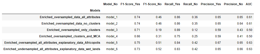
In spatial modeling we used Forest-based Classification and Regression on different datasets with 100 trees. Adding clustering data did not seem to improve the models. Model 1 and Model 2 show very similar results. Model 3 and 4 use only the clustering features and MCAs respectively. They perform well for functional water points but underperform for non-functional ones. For Model 5 and 6 we are using additional layers with over and undersampling. Using explanatory training distance features improves the performance of non-functional water points. The best performer is Model 6 with adding the Ug_Wetlands-extent-and-types1996 layer extracted from Africa Geoportal hosted by Esri4 , followed really closely by model 5 with the Uganda_UrbanAreas_Africapolis layer provided with the initial package. Both layers can be seen in Figure 23 . These models had the highest AUC and Precision.
It is interesting to note that the best two models (5 and 6) use two types of techniques to manage the imbalanced data, yet they arrive at very similar results. Model 5 uses oversampling and Model 6 uses undersampling. Figure 24 shows a map of the results of Model 6. In blue correctly classified points and in orange misclassified points. Figure 25 shows the prediction performance plot for Model 6. Figure 26 shows the prediction performance table for Model5. Table 7 provides a summary of the results for each model for spatial modeling.
Conclusion
Comparison Between Spatial and Non-Spatial Data
After testing different models using enriched data set with ArcGIS Pro’s Random Forest (spatial models) and scikit-learn (non-spatial models), we were able to obtain slightly better results with non-spatial models. This may be because we have more knowledge and tools to tune the non-spatial models. For example, we were able to implement the SMOTE method and other synthetic sampling methods to deal with the unbalanced data.
Working with imbalanced data, we considered the F1, Recall, and Precision scores to be a more accurate representation of the performance of the models. When choosing our model, we are considering higher numbers on the minority labels mentioned above.
Regarding spatial models, we chose Model 6 because it had the best F1, Precision, Recall and AUC on the minority class. Model 5 had very close results with slightly better metrics on the majority class.
In comparison, for the non-spatial models KNN and Random Forest performed best. Random Forest seemed to handle the task slightly better at every sampling method.
We noticed that the spatial analysis produced more consistent results regardless of the sampling method. Non-spatial analysis showed different results based on the sampling method as we mentioned above. If our objective is to have higher Recall, we would suggest Nearest Neighbor Undersampling methods to achieve it. Also, we have to note, that if our goal is high Precision, we would suggest the SVM model. Table 8 shows the summary of the best spatial and non-spatial models.
| Model | Precision | Recall | F-1 | AUC | |||
|---|---|---|---|---|---|---|---|
| Status_Id | 0 | 1 | 0 | 1 | 0 | 1 | |
| SPATIAL | |||||||
| Model 5: Layer Africapolis | 0.65 | 0.67 | 0.42 | 0.84 | 0.51 | 0.75 | 0.63 |
| Model6: Layer Wet lands | 0.66 | 0.67 | 0.42 | 0.83 | 0.52 | 0.73 | 0.63 |
| NON-SPATIAL | |||||||
| Sample traditional oversampling (RF) | 0.66 | 0.79 | 0.5 | 0.88 | 0.57 | 0.83 | 0.689 |
| Sample X10,y10 Edited Nearest Neighbor undersample (RF) | 0.27 | 0.9 | 0.79 | 0.47 | 0.4 | 0.62 | 0.632 |
| Sample X12,y12 Neighborhood cleaning rule (RF) | 0.29 | 0.9 | 0.73 | 0.57 | 0.41 | 0.7 | 0.649 |
| Sample X15,y15 SMOTE+Edited Nearest Neighbor (RF) | 0.36 | 0.88 | 0.54 | 0.77 | 0.44 | 0.82 | 0.658 |
| KNN k=3 | 0.56 | 0.79 | 0.55 | 0.8 | 0.55 | 0.79 | 0.606 |
| Naïve Bayes | 0.3 | 0.81 | 0.05 | 0.97 | 0.08 | 0.88 | 0.51 |
| Dummy Classifier | 0.00 | 0.81 | 0.00 | 1.0 | 0.00 | 0.89 | 0.50 |
Table Non-spatial modeling highlights
Recommendations
Throughout the analysis, we focused on how to predict if a water point is working or not working. Our models for the minority did not perform as desired in predicting them and it made us think that it is almost random which water point is broken and which one is not. As we mentioned at the beginning, for the water technology column, the baseline is “no technology”, and more than 80% of the data had no pump, no kiosk etc. In our dataset only 154 observations were on piped water. The majority was a borehole (36,571), protected spring (27,660), undefined shallow well (18,177) rainwater harvesting (16,620). Assuming that people have access to these water sources, what guarantees that the water is safe to drink? It is a vicious cycle: People cannot afford safe water so they walk hours to get water that might not be potable. The socio-economic impact is dramatic. Because they spend their time going after water, they cannot be employed. Also, they are more likely to get sick from the unhealthy conditions, which would keep them away from work, put a strain on the medical system etc. The real solution would be affordable water through infrastructure, where the quality of the water could be controlled. Strategically build water points within easy reach for everyone.
Lessons Learned
ArcPy and ArcGIS Pro Versus Regular Python:
The main purpose of this project was not only to do data analysis but also to learn how to work with ArcGIS Pro and use ArcPy. We used manly the ArcGIS Pro for both spatial and non-spatial analysis. Our Jupiter notebooks were created inside ArcGIS Pro, we never left this environment. It was easy to see that without the capabilities of ArcGIS Pro we would have missed crucial information. For example, it would have been impossible to distinguish and find the points outside the country’s boundaries. There were many calculations that were at the tip of our fingertip using ArcPy functions, while in regular Python it took several steps and modifications to get the same results. One of the questions we were only able to answer using only ArcPy (creating buffers to be able to calculate how many people were outside easy reach of water as Figure 22). We found the ArcGIS Pro’s GUI was easy and fast to work with, but some calculations when transferred into the notebook using ArcPy took considerable time to run. The under and oversampling was done automatically in ArcGIS while on regular Python we had to create new datasets and then use them in the models. We found that our training from our graduate studies helped a lot in tuning our non-spatial models.
Challenges That We Overcame:
Our first challenge was to quickly understand how to think spatially, how we can use layers on top of each other to extract information. Once learned, we found that some of tasks became very natural and easy. The way we overcome this first challenge was to rewatch lectures, read about the topic and mostly talk it through with each other. It helped a lot when we were coding and debugging together through shared screens.
The rest of the challenges were mostly technical and not about what we needed to do, but how to do it right. For example, improving our data, through enrichment, took considerable time and effort to get the results that we were happy with. It required imputing data to districts with missing data. Also, the enrichment data was district data, we needed point data for within each district. ArcGIS Pro was a big help doing these tasks.
For modeling, we did not want to run every model we were ever thought, but rather use the ones that make sense based on our data exploration and questions (e.g. It would not make sense to run a regression on a classification problem).
References:
Evaluation metrics:
https://medium.com/@klintcho/explaining-precision-and-Recall-c770eb9c69e9
Sampling methods:
https://machinelearningmastery.com/undersampling-algorithms-for-imbalanced-classification/
https://machinelearningmastery.com/undersampling-algorithms-for-imbalanced-classification/
Dimensionality reduction:
https://machinelearningmastery.com/autoencoder-for-classification/
https://blog.keras.io/building-autoencoders-in-keras.html
https://towardsdatascience.com/autoencoder-neural-networks-what-and-how-354cba12bf86
Dealing with unbalanced datasets:
https://bigdata-madesimple.com/dealing-with-unbalanced-class-svm-random-forest-and-decision-tree-in-python/
https://machinelearningmastery.com/cost-sensitive-svm-for-imbalanced-classification/
https://machinelearningmastery.com/one-class-classification-algorithms/
https://machinelearningmastery.com/tactics-to-combat-imbalanced-classes-in-your-machine-learning-dataset/
https://www.kdnuggets.com/2020/04/introduction-k-nearest-neighbour-algorithm-using-examples.html
Picture sources:
https://jssozi.wordpress.com/2010/10/15/water-and-people-in-rural-uganda/
https://www.oregonlive.com/travel/2011/04/your_best_shot_children_carryi.html
https://www.worldvision.org/clean-water-news-stories/long-path-clean-water
Books:
Friedman, Jerome, Trevor Hastie, and Robert Tibshirani. The elements of statistical learning. Vol. 1, no. 10. New York: Springer series in statistics, 2001.
James, Gareth, Daniela Witten, Trevor Hastie, and Robert Tibshirani. An introduction to statistical learning. Vol. 112. New York: springer, 2013.
Christopher M. Bishop. Pattern Recognition and Machine Learning (Information Science and Statistics). Springer-Verlag, Berlin, Heidelberg, 2006
Appendix:
Different datasets for analysis
| Enriched base dataset | Enriched with clusters |
|---|---|
| F_lat_deg | F_lat_deg |
| F_lon_deg | F_lon_deg |
| F_status_id | F_status_id |
| F_water_source_clean | F_water_source_clean |
| F_facility_type | F_facility_type |
| F_install_year | F_install_year |
| management_clean | management_clean |
| water_source_category | water_source_category |
| water_tech_category | water_tech_category |
| Type_of_region | Type_of_region |
| Age | Age |
| ADM1_EN | ADM1_EN |
| UNEMP_CY | UNEMP_CY |
| POPPRM_CY | POPPRM_CY |
| AVGHHSZ_CY | AVGHHSZ_CY |
| Cluster_KModes | |
| HDBS_Cluster | |
| Constrained_Multi_Cluster |
Table . Full Random Forest results an all the sampling methods
| MCA and clusters | Autoencoder and clusters |
|---|---|
| MCA_0 | AE_0 |
| MCA_1 | AE_1 |
| Cluster_KModes | Cluster_KModes |
| HDBS_Cluster | HDBS_Cluster |
| Constrained_Multi_Cluster | Constrained_Multi_Cluster |
Table .Spatial modeling results
Additional Support Plots
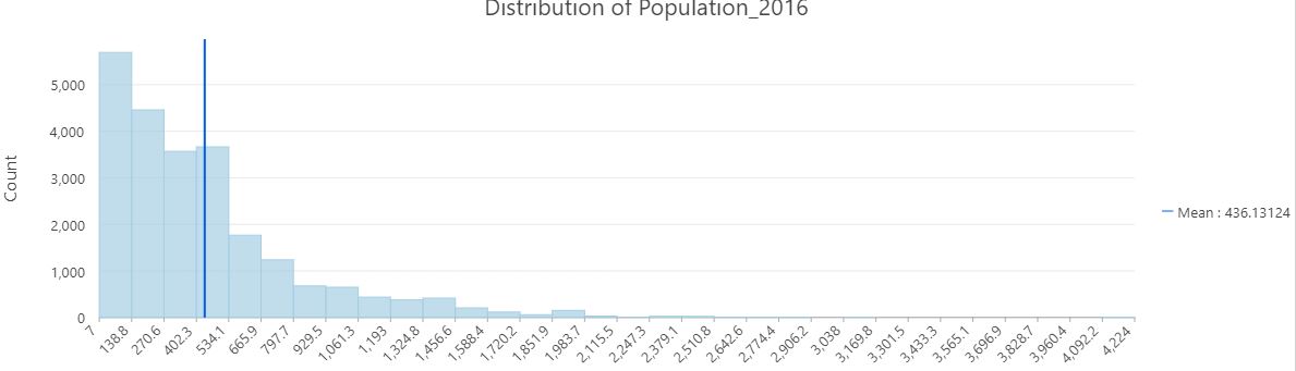
Figure 17 Distribution of population per population point
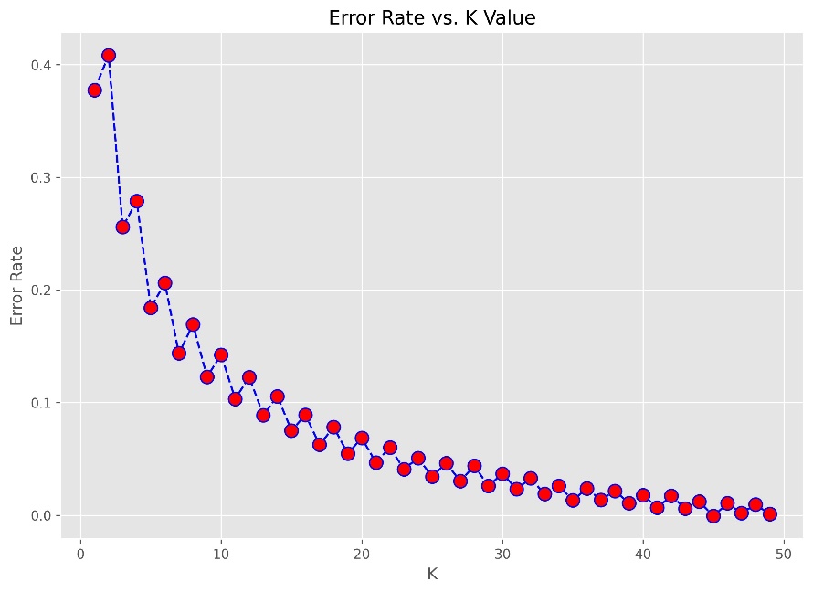
Figure KNN vs Error Rate
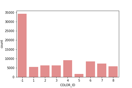
Figure HDBSCAN Cluster allocation
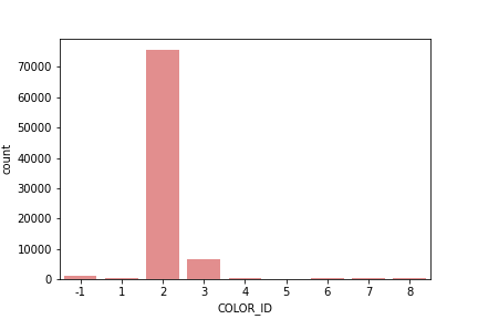
Figure OPTICS Cluster allocation
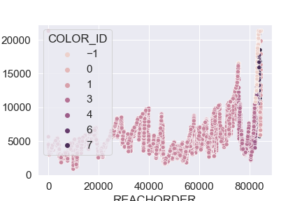
Figure OPTICS reachability plot
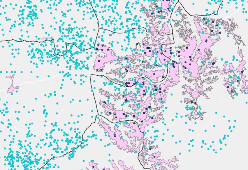
Figure .Selection of rural points outside of Urban layer in light blue
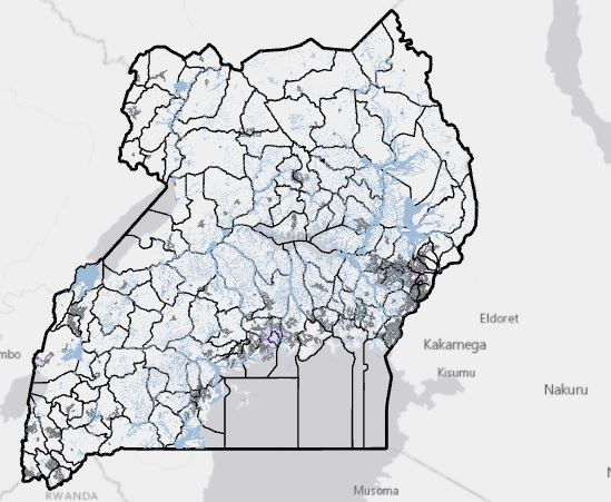
Figure Layer of wetlands in blue and layer of urban areas in pink
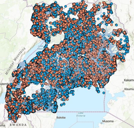
Figure Model 6 classification results using Random Forest undersampled with wet lands layer
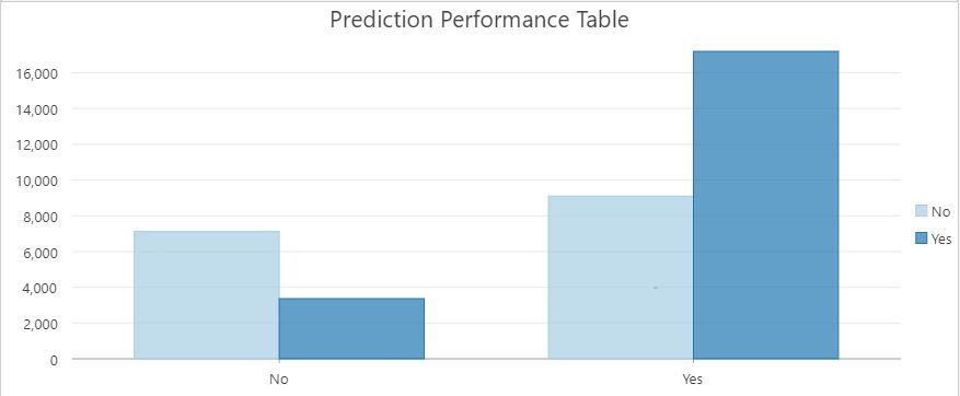
Figure .Model 6 prediction performance table
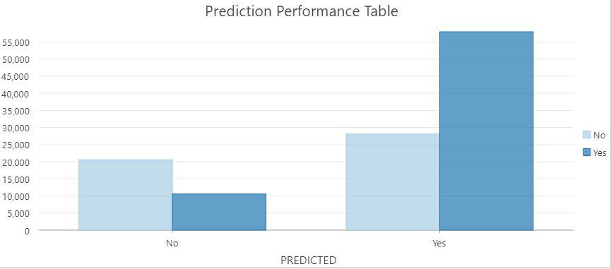
Figure . Model 5 prediction performance table
**
**
Outputs for different models:
Dummy Classifier:
**Same result no matter the sampling**
F1 Score: 0.892
[[ 0 4941]
[ 0 20486]]
precision Recall f1-score support
0 0.00 0.00 0.00 4941
1 0.81 1.00 0.89 20486
accuracy 0.81 25427
macro avg 0.40 0.50 0.45 25427
weighted avg 0.65 0.81 0.72 25427
Accuracy: 0.8056790026349943
Cohen Kappa: 0.000
AUC: 0.500
Naïve Bayes results:
**Sample: Enriched base data, no clusters**
0.7031895229480474
[[ 1739 3202]
[ 4345 16141]]
precision Recall f1-score support
0 0.29 0.35 0.32 4941
1 0.83 0.79 0.81 20486
accuracy 0.70 25427
macro avg 0.56 0.57 0.56 25427
weighted avg 0.73 0.70 0.71 25427
Cohen Kappa: 0.129
AUC: 0.570
**Sample: Enriched base data with clusters**
0.6943013332284579
[[ 1787 3154]
[ 4619 15867]]
precision Recall f1-score support
0 0.28 0.36 0.31 4941
1 0.83 0.77 0.80 20486
accuracy 0.69 25427
macro avg 0.56 0.57 0.56 25427
weighted avg 0.73 0.69 0.71 25427
Cohen Kappa: 0.122
AUC: 0.568
**Sample MCA and clusters**
0.7954143233570614
[[ 83 4858]
[ 344 20142]]
precision Recall f1-score support
0 0.19 0.02 0.03 4941
1 0.81 0.98 0.89 20486
accuracy 0.80 25427
macro avg 0.50 0.50 0.46 25427
weighted avg 0.69 0.80 0.72 25427
Cohen Kappa: 0.000
AUC: 0.500
**Sample autoencoder and clusters**
0.7932905966099029
[[ 230 4711]
[ 545 19941]]
precision Recall f1-score support
0 0.30 0.05 0.08 4941
1 0.81 0.97 0.88 20486
accuracy 0.79 25427
macro avg 0.55 0.51 0.48 25427
weighted avg 0.71 0.79 0.73 25427
Cohen Kappa: 0.029
AUC: 0.510
**Sample traditional oversampling**
0.6394995708721198
[[ 3802 5813]
[ 5108 15571]]
precision Recall f1-score support
0 0.43 0.40 0.41 9615
1 0.73 0.75 0.74 20679
accuracy 0.64 30294
macro avg 0.58 0.57 0.58 30294
weighted avg 0.63 0.64 0.64 30294
Cohen Kappa: 0.151
AUC: 0.574
**Sample X15,y15**
0.6779014433476226
[[ 2000 2941]
[ 5249 15237]]
precision Recall f1-score support
0 0.28 0.40 0.33 4941
1 0.84 0.74 0.79 20486
accuracy 0.68 25427
macro avg 0.56 0.57 0.56 25427
weighted avg 0.73 0.68 0.70 25427
Cohen Kappa: 0.126
AUC: 0.574
Support Vector Machine results:
**Sample: enriched data only**
Accuracy: 0.8093365320328785
[[ 206 4735]
[ 113 20373]]
precision Recall f1-score support
0 0.65 0.04 0.08 4941
1 0.81 0.99 0.89 20486
accuracy 0.81 25427
macro avg 0.73 0.52 0.49 25427
weighted avg 0.78 0.81 0.74 25427
Precision: 0.8114146885454835
Recall: 0.9944840378795274
Cohen Kappa: 0.056
AUC: 0.518
**Sample enriched and clusters**
Accuracy: 0.8094938451252606
[[ 170 4771]
[ 73 20413]]
precision Recall f1-score support
0 0.70 0.03 0.07 4941
1 0.81 1.00 0.89 20486
accuracy 0.81 25427
macro avg 0.76 0.52 0.48 25427
weighted avg 0.79 0.81 0.73 25427
Precision: 0.8105543202033036
Recall: 0.9964365908425266
Cohen Kappa: 0.048
AUC: 0.515
**Sample MCA and clusters**
Accuracy: 0.8063475832776182
[[ 23 4918]
[ 6 20480]]
precision Recall f1-score support
0 0.79 0.00 0.01 4941
1 0.81 1.00 0.89 20486
accuracy 0.81 25427
macro avg 0.80 0.50 0.45 25427
weighted avg 0.80 0.81 0.72 25427
Precision: 0.8063627057248602
Recall: 0.9997071170555502
Cohen Kappa: 0.007
AUC: 0.502
**Sample Autoencoder and clusters**
Accuracy: 0.8061509419121407
[[ 16 4925]
[ 4 20482]]
precision Recall f1-score support
0 0.80 0.00 0.01 4941
1 0.81 1.00 0.89 20486
accuracy 0.81 25427
macro avg 0.80 0.50 0.45 25427
weighted avg 0.80 0.81 0.72 25427
Precision: 0.8061557838390995
Recall: 0.9998047447037001
Cohen Kappa: 0.005
AUC: 0.502
**Sample traditional oversample**
Accuracy: 0.7245989304812834
[[ 2690 6925]
[ 1418 19261]]
precision Recall f1-score support
0 0.65 0.28 0.39 9615
1 0.74 0.93 0.82 20679
accuracy 0.72 30294
macro avg 0.70 0.61 0.61 30294
weighted avg 0.71 0.72 0.69 30294
Precision: 0.7355457114488658
Recall: 0.9314280187629963
Cohen Kappa: 0.249
AUC: 0.606
**Sample X15,y15**
Accuracy: 0.7451527903409761
[[ 2444 2497]
[ 3983 16503]]
precision Recall f1-score support
0 0.38 0.49 0.43 4941
1 0.87 0.81 0.84 20486
accuracy 0.75 25427
macro avg 0.62 0.65 0.63 25427
weighted avg 0.77 0.75 0.76 25427
Precision: 0.868578947368421
Recall: 0.8055745387093625
Cohen Kappa: 0.269
AUC: 0.650
KNN results:
**For k=4 and only enriched data**
[[ 1940 3001]
[ 3101 17385]]
precision Recall f1-score support
0 0.38 0.39 0.39 4941
1 0.85 0.85 0.85 20486
accuracy 0.76 25427
macro avg 0.62 0.62 0.62 25427
weighted avg 0.76 0.76 0.76 25427
Cohen Kappa: 0.239
AUC: 0.621
**Sample k=4 for enriched with clusters**
[[ 1984 2957]
[ 3158 17328]]
precision Recall f1-score support
0 0.39 0.40 0.39 4941
1 0.85 0.85 0.85 20486
accuracy 0.76 25427
macro avg 0.62 0.62 0.62 25427
weighted avg 0.76 0.76 0.76 25427
Cohen Kappa: 0.244
AUC: 0.624
**Sample MCA and clusters, k=4**
[[ 1923 3018]
[ 3031 17455]]
precision Recall f1-score support
0 0.39 0.39 0.39 4941
1 0.85 0.85 0.85 20486
accuracy 0.76 25427
macro avg 0.62 0.62 0.62 25427
weighted avg 0.76 0.76 0.76 25427
Cohen Kappa: 0.241
AUC: 0.621
**Sample Autoencoder and clusters k=3**
[[ 1450 3491]
[ 1958 18528]]
precision Recall f1-score support
0 0.43 0.29 0.35 4941
1 0.84 0.90 0.87 20486
accuracy 0.79 25427
macro avg 0.63 0.60 0.61 25427
weighted avg 0.76 0.79 0.77 25427
Cohen Kappa: 0.224
AUC: 0.599
**Sample traditional oversampeling**
[[ 5243 4372]
[ 4154 16525]]
precision Recall f1-score support
0 0.56 0.55 0.55 9615
1 0.79 0.80 0.79 20679
accuracy 0.72 30294
macro avg 0.67 0.67 0.67 30294
weighted avg 0.72 0.72 0.72 30294
Cohen Kappa: 0.347
AUC: 0.672
**Sample X15,y15, k=40**
[[ 2751 2190]
[ 5133 15353]]
precision Recall f1-score support
0 0.35 0.56 0.43 4941
1 0.88 0.75 0.81 20486
accuracy 0.71 25427
macro avg 0.61 0.65 0.62 25427
weighted avg 0.77 0.71 0.73 25427
Cohen Kappa: 0.250
AUC: 0.653
One-Class SVM results:
**Sample: enriched data only:**
F1 Score: 0.888
[[ 107 4834]
[ 266 20220]]
precision Recall f1-score support
-1 0.29 0.02 0.04 4941
1 0.81 0.99 0.89 20486
accuracy 0.80 25427
macro avg 0.55 0.50 0.46 25427
weighted avg 0.71 0.80 0.72 25427
Cohen Kappa: 0.013
AUC: 0.504
**Sample enriched and clusters**
F1 Score: 0.889
[[ 101 4840]
[ 238 20248]]
precision Recall f1-score support
-1 0.30 0.02 0.04 4941
1 0.81 0.99 0.89 20486
accuracy 0.80 25427
macro avg 0.55 0.50 0.46 25427
weighted avg 0.71 0.80 0.72 25427
Cohen Kappa: 0.014
AUC: 0.504
**Sample MCA and clusters***
F1 Score: 0.889
[[ 105 4836]
[ 226 20260]]
precision Recall f1-score support
-1 0.32 0.02 0.04 4941
1 0.81 0.99 0.89 20486
accuracy 0.80 25427
macro avg 0.56 0.51 0.46 25427
weighted avg 0.71 0.80 0.72 25427
Cohen Kappa: 0.016
AUC: 0.505
**Sample autoencoder and clusters**
F1 Score: 0.889
[[ 80 4861]
[ 194 20292]]
precision Recall f1-score support
-1 0.29 0.02 0.03 4941
1 0.81 0.99 0.89 20486
accuracy 0.80 25427
macro avg 0.55 0.50 0.46 25427
weighted avg 0.71 0.80 0.72 25427
Cohen Kappa: 0.010
AUC: 0.503
Isolation Forest results:
**Sample: enriched data only:**
F1 Score: 0.756
[[ 1724 3217]
[ 6081 14405]]
precision Recall f1-score support
-1 0.22 0.35 0.27 4941
1 0.82 0.70 0.76 20486
accuracy 0.63 25427
macro avg 0.52 0.53 0.51 25427
weighted avg 0.70 0.63 0.66 25427
Cohen Kappa: 0.043
AUC: 0.526
**Sample enriched and clusters**
F1 Score: 0.755
[[ 1713 3228]
[ 6115 14371]]
precision Recall f1-score support
-1 0.22 0.35 0.27 4941
1 0.82 0.70 0.75 20486
accuracy 0.63 25427
macro avg 0.52 0.52 0.51 25427
weighted avg 0.70 0.63 0.66 25427
Cohen Kappa: 0.039
AUC: 0.524
**Sample MCA and clusters***
F1 Score: 0.750
[[ 1633 3308]
[ 6205 14281]]
precision Recall f1-score support
-1 0.21 0.33 0.26 4941
1 0.81 0.70 0.75 20486
accuracy 0.63 25427
macro avg 0.51 0.51 0.50 25427
weighted avg 0.69 0.63 0.65 25427
Cohen Kappa: 0.023
AUC: 0.514
**Sample autoencoder and clusters**
F1 Score: 0.759
[[ 1789 3152]
[ 6016 14470]]
precision Recall f1-score support
-1 0.23 0.36 0.28 4941
1 0.82 0.71 0.76 20486
accuracy 0.64 25427
macro avg 0.53 0.53 0.52 25427
weighted avg 0.71 0.64 0.67 25427
Cohen Kappa: 0.056
AUC: 0.534